Interpolación - Scipy#
import matplotlib.pyplot as plt
import numpy as np
Interpolación#
Fundamentos#
La interpolación consiste en encontrar una función \(f(x)\) tal que, dadas las abscisas $\( x_0,x_1,\cdots,x_{n-1} \)\( y sus correspondientes valores de ordenadas \)\( y_0,y_1,\cdots,y_{n-1} \)\( se verifique que: \)\( f(x_i) = y_i \;\;\; \textrm{para cualquier} \;\; 0\le i < n \)$
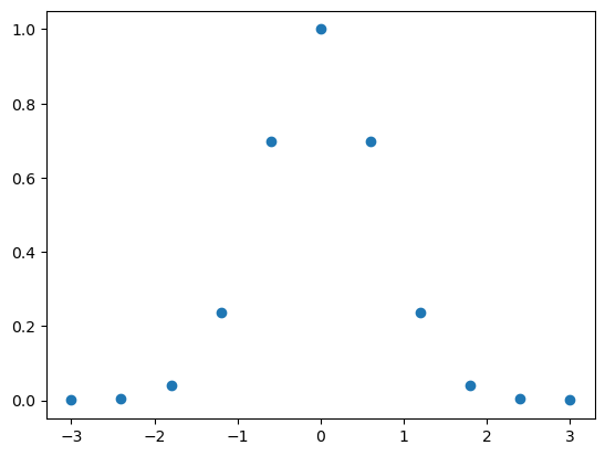
Si lo pensamos en el plano, queremos buscar una curva \(f(x)\) que pase por todos los puntos \((x_i,y_i)\), con \(0\le i < n\).
xData = np.linspace(-3,3,11)
xData
array([-3. , -2.4, -1.8, -1.2, -0.6, 0. , 0.6, 1.2, 1.8, 2.4, 3. ])
yData = np.array([1.23409804e-04, 3.15111160e-03, 3.91638951e-02, 2.36927759e-01,
       6.97676326e-01, 1.00000000e+00, 6.97676326e-01, 2.36927759e-01,
       3.91638951e-02, 3.15111160e-03, 1.23409804e-04])
yData
array([1.23409804e-04, 3.15111160e-03, 3.91638951e-02, 2.36927759e-01,
       6.97676326e-01, 1.00000000e+00, 6.97676326e-01, 2.36927759e-01,
       3.91638951e-02, 3.15111160e-03, 1.23409804e-04])
plt.plot(xData,yData, marker = 'o',linestyle = 'None')
plt.show()
La interpolación tiene dos etapas:
Encontrar la función interpoladora \(f(x)\)
Evaluar la función interpoladora en los valores deseados
Interpolación polinomial (de Newton)#
Por supuesto que es extremadamente difícil encontrar una función \(f(x)\) general para cualquier cantidad de puntos \((x_i,y_i)\) dados como datos. Por eso se utilizan polinomios de distinto grado para satisfacer las condiciones de la interpolación.
Una de las posibles formas funcionales corresponde a los polinomios de Newton, definidos como:
Por ejemplo, el polinomio de Newton para ajustar tres puntos \((x_0,y_0)\), \((x_1,y_1)\) y \((x_2,y_2)\) es:
Y en este caso, tenemos que buscar los valores \(a_0, a_1, a_2\) de forma tal que:
\begin{align} y_0 &= P_2(x_0) \ y_1 &= P_2(x_1) \ y_2 &= P_2(x_2) \end{align} Reemplazando:
\begin{align} y_0 &= a_0 \ y_1 &= a_0 + a_1 (x_1 - x_0) \ y_2 &= a_0 + a_1 (x_2 - x_0) + a_2 (x_2-x_0)(x_2-x_1) \end{align}
Este sistema es sencillo de resolver, empezando por la primer ecuación
continuando por la segunda: \begin{align} y_1 &= y_0 + a_1 (x_1 - x_0) \ y_1 - y_0 &= a_1 (x_1 - x_0) \ a_1 &= \frac{y_1 - y_0 }{x_1 - x_0} \end{align}
y finalmente reemplazando \(a_0\) y \(a_1\) en la tercera ecuación: \begin{align} y_2 &= a_0 + a_1 (x_2 - x_0) + a_2 (x_2-x_0)(x_2-x_1) \ y_2 &= y_0 + \frac{y_1 - y_0 }{x_1 - x_0} (x_2 - x_0) + a_2 (x_2-x_0)(x_2-x_1) \ a_2 (x_2-x_0)(x_2-x_1) &= y_2 - y_0 - \frac{y_1 - y_0 }{x_1 - x_0} (x_2 - x_0) \end{align} con
Simplificando:
Los polinomios están construidos de forma tal que:
Son fáciles de evaluar numéricamente#
Por ejemplo, en el caso de \(P_3(x)\):
\begin{align} P_3(x) &= a_0 + a_1 (x - x_0) + a_2 (x-x_0)(x-x_1) + a_3 (x-x_0)(x-x_1)(x-x_2)\ &= a_0 + (x - x_0) \left[ a_1 + a_2 (x - x_1) + a_3 (x-x_1)(x-x_2) \right] \ &= a_0 + (x - x_0) \left{ a_1 + (x - x_1) \left[a_2 + a_3 (x-x_2)\right] \right} \end{align}
que si se evalúa desde atrás hacia adelante, queda: \begin{align} Q_0(x) &= a_3\ Q_1(x) &= a_2 + Q_0(x) (x - x_2) \ Q_2(x) &= a_1 + Q_1(x) (x - x_1) \ Q_3(x) &= a_0 + Q_2(x) (x - x_0) \end{align} y obviamente, \(Q_3(x) = P_3(x)\)
En general
Encontrar los valores de los coeficientes es sencillo#
Como vimos antes, el sistema de ecuaciones a resolver es triangular, y se resuelve fácilmente.
Ejemplo#
Copiamos el módulo newtonPoly.py en el directorio de trabajo.
import newtonPoly as newton
---------------------------------------------------------------------------
ModuleNotFoundError                       Traceback (most recent call last)
Cell In[5], line 1
----> 1 import newtonPoly as newton

ModuleNotFoundError: No module named 'newtonPoly'
help(newton)
Help on module newtonPoly:

NAME
    newtonPoly

DESCRIPTION
    p = evalPoly(a,xData,x).
    Evaluates Newton's polynomial p at x. The coefficient
    vector 'a' can be computed by the function 'coeffts'.

    a = coeffts(xData,yData).
    Computes the coefficients of Newton's polynomial.

FUNCTIONS
    coeffts(xData, yData)

    evalPoly(a, xData, x)

FILE
    /Users/flavioc/Library/Mobile Documents/com~apple~CloudDocs/Documents/cursos/taller de informática/2021/newtonPoly.py
Evaluemos los coeficientes para los datos que teníamos antes
a = newton.coeffts(xData,yData)
a
array([ 0.00012341,  0.00504617,  0.04581261,  0.09935648, -0.00885172,
       -0.05305972,  0.02955858, -0.00406494, -0.00248136,  0.00169219,
       -0.00056406])
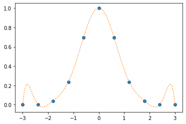
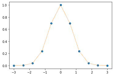
Para graficar, generamos una grilla densa
xpoly = np.linspace(-3,3,100)
y evaluamos el polinomio en todos esos puntos
ypoly = newton.evalPoly(a,xData,xpoly)
plt.plot(xData,yData, marker = 'o',linestyle = 'None')
plt.plot(xpoly,ypoly,linestyle = 'dotted')
plt.show()
xpoly = np.linspace(-4,4,100)
ypoly = newton.evalPoly(a,xData,xpoly)
plt.plot(xData,yData, marker = 'o',linestyle = 'None')
plt.plot(xpoly,ypoly,linestyle = 'dotted')
plt.show()
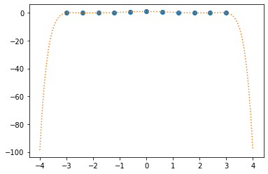
Interpolación a trozos (piecewise interpolation)#
Como se ve en el ejemplo anterior, es difícil encontrar una sola función que pueda funcionar como interpolador, y que a su vez tenga una forma suave. Por eso se usan métodos de interpolación a trozos. Para eso, se define un conjunto de funciones \(\{f(x)\}\) de modo tal que cada una de ellas se use para interpolar sólo un sector particular del dominio \(x_0, x_1, \cdots, x_n\).
Una vez realizada la interpolación, esto es, una vez conocidas las funciones \(\{f(x)\}\), la evaluación de dichas funciones (es decir, la etapa 2. descripta antes) requiere a su vez de dos pasos:
Encontrar qué función se debe utilizar de acuerdo al valor de \(x\)
Evaluar la función seleccionada en \(x\)
El primer paso se conoce habitualmente como lookup.
Veremos en detalle el ejemplo de la interpolación lineal.
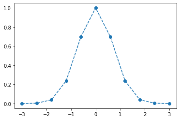
Interpolación lineal#
Sin dudas la interpolación lineal es la más usada en física médica. Consiste en definir funciones lineales que se utilizarán para interpolar todos los valores de \(x\) entre dos abscisas contiguas \(x_i\) y \(x_{i+1}\):
En efecto,
mientras que
Es decir que la función \(p_i(x)\) verifica la condición de interpolación en \(x_i\) y \(x_{i+1}\).
plt.plot(xData,yData, marker = 'o',linestyle = 'dashed')
plt.show()
Splines cúbicos#
El otro tipo de interpolación utilizado frecuentemente corresponde a los denominados splines cúbicos. Éstos son polinomios de tercer orden que se construyen entre dos abscisas contiguas \(x_i\) y \(x_{i+1}\). Sin embargo, en estos casos, además de las condiciones
\begin{align} y_i &= f(x_i) \ y_{i+1} &= f(x_{i+1}), \end{align}
es necesario imponer condiciones extras dado que un polinomio de orden 3 tiene 4 coeficientes a determinar. En general se pueden imponer condiciones sobre las derivadas primeras de la función: \begin{align} y’i &= f’(x_i) \ y’{i+1} &= f’(x_{i+1}), \end{align} O el caso más común, de los splines naturales en los que se pide \begin{align} f’’(x_i) &= 0 \ f’’(x_{i+1}) &= 0. \end{align}
El álgebra para obtenerlos es algo engorrosa, así que la pueden consultar por ahí.
Módulos al rescate: Scipy#
Afortunadamente, existe un módulo que hace este tipo de cosas, y muchas más. Se trata del módulo scipy. En particular, usaremos el submódulo interpolate:
from scipy.interpolate import interp1d
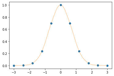
Interpolación lineal#
f_lineal = interp1d(xData,yData)  # Por defecto, la interpolación de interp1d es lineal
xs = np.linspace(-3,3,100)
ylineal = f_lineal(xs)

plt.plot(xData,yData, marker = 'o',linestyle = 'None')
plt.plot(xs,ylineal,linestyle = 'dotted')
plt.show()
print(f_lineal(0.5))
0.7480636049999998
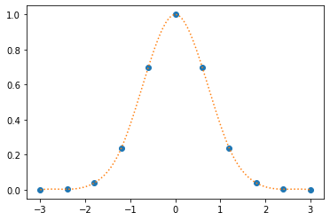
Interpolación cuadrática#
f_quad = interp1d(xData,yData,kind='quadratic') # Definiendo el parámetro kind, se obtienen otras interpolaciones
yquad = f_quad(xs)

plt.plot(xData,yData, marker = 'o',linestyle = 'None')
plt.plot(xs,yquad,linestyle = 'dotted')
plt.show()
Interpolación cúbica#
f_cubic = interp1d(xData,yData,kind='cubic') # Definiendo el parámetro kind, se obtienen otras interpolaciones
ycubic = f_cubic(xs)

plt.plot(xData,yData, marker = 'o',linestyle = 'None')
plt.plot(xs,ycubic,linestyle = 'dotted')
plt.show()
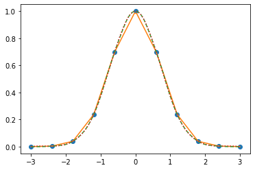
Graficamos todos los ajustes juntos:
plt.plot(xData,yData, marker = 'o',linestyle = 'None')
plt.plot(xs,ylineal,linestyle = 'solid')
plt.plot(xs,yquad,linestyle = 'dashed')
plt.plot(xs,ycubic,linestyle = 'dotted')
plt.show()
Fiteo de curvas#
Otra tarea frecuente es ajustar parámetros de una función objetivo a partir de un dataset de puntos conocidos.
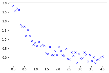
Supongamos que tenemos una serie de datos medidos
xdata = np.array([0.        , 0.08163265, 0.16326531, 0.24489796, 0.32653061,
       0.40816327, 0.48979592, 0.57142857, 0.65306122, 0.73469388,
       0.81632653, 0.89795918, 0.97959184, 1.06122449, 1.14285714,
       1.2244898 , 1.30612245, 1.3877551 , 1.46938776, 1.55102041,
       1.63265306, 1.71428571, 1.79591837, 1.87755102, 1.95918367,
       2.04081633, 2.12244898, 2.20408163, 2.28571429, 2.36734694,
       2.44897959, 2.53061224, 2.6122449 , 2.69387755, 2.7755102 ,
       2.85714286, 2.93877551, 3.02040816, 3.10204082, 3.18367347,
       3.26530612, 3.34693878, 3.42857143, 3.51020408, 3.59183673,
       3.67346939, 3.75510204, 3.83673469, 3.91836735, 4.        ])

ydata = np.array([ 2.86176601,  2.57905526,  2.70036593,  2.63066436,  1.8035502 ,
        1.69507105,  1.71332572,  1.19968728,  1.53954472,  1.19541914,
        0.90611978,  0.7115336 ,  0.80780086,  0.64485915,  0.85535322,
        0.61878794,  0.69171233,  0.64694833,  0.23714098,  0.18498906,
        0.58324814,  0.13810763,  0.12359655,  0.33529197,  0.15601467,
        0.59733706,  0.35817119,  0.11824581,  0.08785438,  0.49333643,
       -0.09737018, -0.11026946,  0.27281943,  0.10931485,  0.27558412,
       -0.27575616,  0.21938698, -0.05069495, -0.03916167,  0.28574475,
        0.15924156, -0.21736918,  0.1431817 , -0.1881811 ,  0.00901724,
       -0.31409179, -0.11894992, -0.11414616,  0.01245554,  0.04917944])
print(len(ydata))
50
plt.plot(xdata, ydata, 'xb', label='DATOS')
plt.show()
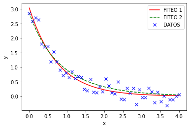
def func(x, a, b, c, d):
    return a * np.exp(-b * x) + c * np.exp(-d * x)
from scipy.optimize import curve_fit


popt, pcov = curve_fit(func, xdata, ydata)
print(popt)

y1 = func(xdata, popt[0],popt[1],popt[2],popt[3])
#
# Una forma compacta de crear y1 es:
# y1 = func(xdata, *popt)
# en lugar de 'desenrollar popt en sus componentes [0]..[3]

plt.plot(xdata, y1, 'r-', label='FITEO 1')

popt, pcov = curve_fit(func, xdata, ydata, bounds=(0, [3., 1., 0.5, 4.]))
y2 = func(xdata, *popt)
plt.plot(xdata, y2, 'g--', label='FITEO 2')

plt.plot(xdata, ydata, 'xb', label='DATOS')
plt.xlabel('x')
plt.ylabel('y')
plt.legend()
plt.show()
[1.33780096 1.30826848 1.69846325 1.30827681]
help(curve_fit)
Help on function curve_fit in module scipy.optimize.minpack:

curve_fit(f, xdata, ydata, p0=None, sigma=None, absolute_sigma=False, check_finite=True, bounds=(-inf, inf), method=None, jac=None, **kwargs)
    Use non-linear least squares to fit a function, f, to data.

    Assumes ``ydata = f(xdata, *params) + eps``.

    Parameters
    ----------
    f : callable
        The model function, f(x, ...). It must take the independent
        variable as the first argument and the parameters to fit as
        separate remaining arguments.
    xdata : array_like or object
        The independent variable where the data is measured.
        Should usually be an M-length sequence or an (k,M)-shaped array for
        functions with k predictors, but can actually be any object.
    ydata : array_like
        The dependent data, a length M array - nominally ``f(xdata, ...)``.
    p0 : array_like, optional
        Initial guess for the parameters (length N). If None, then the
        initial values will all be 1 (if the number of parameters for the
        function can be determined using introspection, otherwise a
        ValueError is raised).
    sigma : None or M-length sequence or MxM array, optional
        Determines the uncertainty in `ydata`. If we define residuals as
        ``r = ydata - f(xdata, *popt)``, then the interpretation of `sigma`
        depends on its number of dimensions:

            - A 1-D `sigma` should contain values of standard deviations of
              errors in `ydata`. In this case, the optimized function is
              ``chisq = sum((r / sigma) ** 2)``.

            - A 2-D `sigma` should contain the covariance matrix of
              errors in `ydata`. In this case, the optimized function is
              ``chisq = r.T @ inv(sigma) @ r``.

              .. versionadded:: 0.19

        None (default) is equivalent of 1-D `sigma` filled with ones.
    absolute_sigma : bool, optional
        If True, `sigma` is used in an absolute sense and the estimated parameter
        covariance `pcov` reflects these absolute values.

        If False (default), only the relative magnitudes of the `sigma` values matter.
        The returned parameter covariance matrix `pcov` is based on scaling
        `sigma` by a constant factor. This constant is set by demanding that the
        reduced `chisq` for the optimal parameters `popt` when using the
        *scaled* `sigma` equals unity. In other words, `sigma` is scaled to
        match the sample variance of the residuals after the fit. Default is False.
        Mathematically,
        ``pcov(absolute_sigma=False) = pcov(absolute_sigma=True) * chisq(popt)/(M-N)``
    check_finite : bool, optional
        If True, check that the input arrays do not contain nans of infs,
        and raise a ValueError if they do. Setting this parameter to
        False may silently produce nonsensical results if the input arrays
        do contain nans. Default is True.
    bounds : 2-tuple of array_like, optional
        Lower and upper bounds on parameters. Defaults to no bounds.
        Each element of the tuple must be either an array with the length equal
        to the number of parameters, or a scalar (in which case the bound is
        taken to be the same for all parameters). Use ``np.inf`` with an
        appropriate sign to disable bounds on all or some parameters.

        .. versionadded:: 0.17
    method : {'lm', 'trf', 'dogbox'}, optional
        Method to use for optimization. See `least_squares` for more details.
        Default is 'lm' for unconstrained problems and 'trf' if `bounds` are
        provided. The method 'lm' won't work when the number of observations
        is less than the number of variables, use 'trf' or 'dogbox' in this
        case.

        .. versionadded:: 0.17
    jac : callable, string or None, optional
        Function with signature ``jac(x, ...)`` which computes the Jacobian
        matrix of the model function with respect to parameters as a dense
        array_like structure. It will be scaled according to provided `sigma`.
        If None (default), the Jacobian will be estimated numerically.
        String keywords for 'trf' and 'dogbox' methods can be used to select
        a finite difference scheme, see `least_squares`.

        .. versionadded:: 0.18
    kwargs
        Keyword arguments passed to `leastsq` for ``method='lm'`` or
        `least_squares` otherwise.

    Returns
    -------
    popt : array
        Optimal values for the parameters so that the sum of the squared
        residuals of ``f(xdata, *popt) - ydata`` is minimized.
    pcov : 2-D array
        The estimated covariance of popt. The diagonals provide the variance
        of the parameter estimate. To compute one standard deviation errors
        on the parameters use ``perr = np.sqrt(np.diag(pcov))``.

        How the `sigma` parameter affects the estimated covariance
        depends on `absolute_sigma` argument, as described above.

        If the Jacobian matrix at the solution doesn't have a full rank, then
        'lm' method returns a matrix filled with ``np.inf``, on the other hand
        'trf'  and 'dogbox' methods use Moore-Penrose pseudoinverse to compute
        the covariance matrix.

    Raises
    ------
    ValueError
        if either `ydata` or `xdata` contain NaNs, or if incompatible options
        are used.

    RuntimeError
        if the least-squares minimization fails.

    OptimizeWarning
        if covariance of the parameters can not be estimated.

    See Also
    --------
    least_squares : Minimize the sum of squares of nonlinear functions.
    scipy.stats.linregress : Calculate a linear least squares regression for
                             two sets of measurements.

    Notes
    -----
    With ``method='lm'``, the algorithm uses the Levenberg-Marquardt algorithm
    through `leastsq`. Note that this algorithm can only deal with
    unconstrained problems.

    Box constraints can be handled by methods 'trf' and 'dogbox'. Refer to
    the docstring of `least_squares` for more information.

    Examples
    --------
    >>> import matplotlib.pyplot as plt
    >>> from scipy.optimize import curve_fit

    >>> def func(x, a, b, c):
    ...     return a * np.exp(-b * x) + c

    Define the data to be fit with some noise:

    >>> xdata = np.linspace(0, 4, 50)
    >>> y = func(xdata, 2.5, 1.3, 0.5)
    >>> np.random.seed(1729)
    >>> y_noise = 0.2 * np.random.normal(size=xdata.size)
    >>> ydata = y + y_noise
    >>> plt.plot(xdata, ydata, 'b-', label='data')

    Fit for the parameters a, b, c of the function `func`:

    >>> popt, pcov = curve_fit(func, xdata, ydata)
    >>> popt
    array([ 2.55423706,  1.35190947,  0.47450618])
    >>> plt.plot(xdata, func(xdata, *popt), 'r-',
    ...          label='fit: a=%5.3f, b=%5.3f, c=%5.3f' % tuple(popt))

    Constrain the optimization to the region of ``0 <= a <= 3``,
    ``0 <= b <= 1`` and ``0 <= c <= 0.5``:

    >>> popt, pcov = curve_fit(func, xdata, ydata, bounds=(0, [3., 1., 0.5]))
    >>> popt
    array([ 2.43708906,  1.        ,  0.35015434])
    >>> plt.plot(xdata, func(xdata, *popt), 'g--',
    ...          label='fit: a=%5.3f, b=%5.3f, c=%5.3f' % tuple(popt))

    >>> plt.xlabel('x')
    >>> plt.ylabel('y')
    >>> plt.legend()
    >>> plt.show()
print(pcov)
perr = np.sqrt(np.diag(pcov))
perr
[[  4.15854294   0.76302348  -4.02901848  14.17297729]
 [  0.76302348   0.14611409  -0.74263071   2.49384224]
 [ -4.02901848  -0.74263071   3.93319959 -13.52705136]
 [ 14.17297729   2.49384224 -13.52705136  52.10488222]]
array([2.03925058, 0.38224873, 1.98322959, 7.21837116])