Imágenes médicas - DICOM#
El standard DICOM#
Para facilitar la intercomunicación entre distintas modalidades de diagnóstico por imágenes, se creó en 1993 el formato DICOM (Digital Imaging and Communications in Medicine). Este es un standard que define cómo guardar la información de una imagen, series de imágenes e incluso videos (cines), junto con datos relevantes de la misma, datos del paciente, del centro médico, de la modalidad específica de diagnóstico, etc.
La definición del standard es extensísima (pueden consultarla en https://www.dicomstandard.org/current), dado que incluye un enorme abanico de posibles tipos de datos.
Esencialmente, un archivo DICOM está estructurado en una lista de TAGS que se componen de la siguiente manera:
Dos números hexadecimales (denominados Grupo y Elemento) que identifican el atributo de la imagen. Cada atributo tiene un nombre asociado, que es el que se utiliza generalmente para acceder al mismo. Por ejemplo
(0008, 0060) Modality
corresponde al grupo 0008, elemento 0006 que describe el atributo Modalidad de la imagen.
Dos letras (Value Representation) que indican el tipo de dato que se está guardando en el tag, por ejemplo
‘SH’ para short strings (hasta 16 caracteres)
‘US’ para enteros sin signo (enteros mayores o iguales que cero, usando 2 bytes)
‘SQ’ para secuencias de otros tags
El valor específico del atributo en sí.
Entonces, un tag completo sería
(0008, 0080) Institution Name LO: 'INTECNUS'
Recomendamos usar la página https://dicom.innolitics.com/ciods para explorar los tag DICOM, dado que la página del standard es compleja para buscar información
Afortunadamente, la gran mayoría de los lenguajes provee de bibliotecas para trabajar con archivos DICOM. Python no es una excepción, y usa el módulo pydicom.
Instalando pydicom#
Desafortunadamente, pydicom no viene instalado por defecto en Anaconda. Veamos cómo instalarlo.
Correr la línea de comando de miniconda.
En la línea de comando,
conda install -c conda-forge pydicom
Usando pydicom#
Una vez instalado pydicom, es posible usarlo como un módulo cualquiera. La documentación está acá: https://pydicom.github.io/pydicom/stable/index.html
Es importante mencionar que, además de poder acceder a todos los tags DICOM de un archivo,
pydicomademás guarda información del archivo en sus propias variables, para facilitar el acceso a las mismas.
import matplotlib.pyplot as plt
import numpy as np
import pydicom

#
#    pydicom provee algunos datos de ejemplo, que se pueden importar así:
#
# from pydicom.data import get_testdata_files
Abrir un archivo DICOM#
DCM = pydicom.dcmread(r'../Assets/CT/IM-0001-0200-0001.dcm')
---------------------------------------------------------------------------
FileNotFoundError                         Traceback (most recent call last)
Cell In[2], line 1
----> 1 DCM = pydicom.dcmread(r'../Assets/CT/IM-0001-0200-0001.dcm')

File /opt/miniconda3/lib/python3.9/site-packages/pydicom/filereader.py:993, in dcmread(fp, defer_size, stop_before_pixels, force, specific_tags)
    991     caller_owns_file = False
    992     logger.debug("Reading file '{0}'".format(fp))
--> 993     fp = open(fp, 'rb')
    994 elif fp is None or not hasattr(fp, "read") or not hasattr(fp, "seek"):
    995     raise TypeError("dcmread: Expected a file path or a file-like, "
    996                     "but got " + type(fp).__name__)

FileNotFoundError: [Errno 2] No such file or directory: '../Assets/CT/IM-0001-0200-0001.dcm'
type(DCM)
pydicom.dataset.FileDataset
DCM
(0008, 0005) Specific Character Set              CS: 'ISO_IR 100'
(0008, 0008) Image Type                          CS: ['ORIGINAL', 'PRIMARY', 'AXIAL']
(0008, 0012) Instance Creation Date              DA: '20191106'
(0008, 0013) Instance Creation Time              TM: '164949'
(0008, 0016) SOP Class UID                       UI: CT Image Storage
(0008, 0018) SOP Instance UID                    UI: 1.2.840.113619.2.290.3.1225403042.932.1573045470.721.200
(0008, 0020) Study Date                          DA: '20191106'
(0008, 0021) Series Date                         DA: '20191106'
(0008, 0022) Acquisition Date                    DA: '20191106'
(0008, 0023) Content Date                        DA: '20191106'
(0008, 0030) Study Time                          TM: '164219'
(0008, 0031) Series Time                         TM: '164539'
(0008, 0032) Acquisition Time                    TM: '164650.808161'
(0008, 0033) Content Time                        TM: '164949'
(0008, 0050) Accession Number                    SH: '2473501'
(0008, 0060) Modality                            CS: 'CT'
(0008, 0070) Manufacturer                        LO: 'GE MEDICAL SYSTEMS'
(0008, 0080) Institution Name                    LO: 'INTECNUS'
(0008, 0090) Referring Physician's Name          PN: '0'
(0008, 1010) Station Name                        SH: 'petct'
(0008, 1030) Study Description                   LO: 'PET CUERPO COMPLETO-'
(0008, 103e) Series Description                  LO: 'Standard/Full'
(0008, 1050) Performing Physician's Name         PN: '"'
(0008, 1060) Name of Physician(s) Reading Study  PN: 'VENTIMIGLIA, ROMINA'
(0008, 1070) Operators' Name                     PN: 'CC'
(0008, 1090) Manufacturer's Model Name           LO: 'Discovery 710'
(0008, 1140)  Referenced Image Sequence   1 item(s) ----
   (0008, 1150) Referenced SOP Class UID            UI: CT Image Storage
   (0008, 1155) Referenced SOP Instance UID         UI: 1.2.840.113619.2.290.3.1225403042.932.1573045470.333.2
   ---------
(0009, 0010) Private Creator                     LO: 'GEMS_IDEN_01'
(0009, 1001) [Full fidelity]                     LO: 'CT_LIGHTSPEED'
(0009, 1002) [Suite id]                          SH: 'CT83'
(0009, 1004) [Product id]                        SH: 'Discovery 710'
(0009, 1027) [Image actual date]                 SL: 1573058739
(0009, 10e3) [Equipment UID]                     UI: ''
(0010, 0010) Patient's Name                      PN: 'PET CT INTECNUS'
(0010, 0020) Patient ID                          LO: '16682827'
(0010, 0030) Patient's Birth Date                DA: '19641026'
(0010, 0040) Patient's Sex                       CS: 'F'
(0010, 1000) Other Patient IDs                   LO: ''
(0010, 1010) Patient's Age                       AS: '055Y'
(0010, 1020) Patient's Size                      DS: "1.62"
(0010, 1030) Patient's Weight                    DS: "65.0"
(0010, 21b0) Additional Patient History          LT: ''
(0018, 0022) Scan Options                        CS: 'HELICAL MODE'
(0018, 0050) Slice Thickness                     DS: "2.500000"
(0018, 0060) KVP                                 DS: "120"
(0018, 0088) Spacing Between Slices              DS: "3.270000"
(0018, 0090) Data Collection Diameter            DS: "500.000000"
(0018, 1020) Software Version(s)                 LO: 'pet_coreload.87'
(0018, 1030) Protocol Name                       LO: '10.1 PET/CT FDG + TORAX'
(0018, 1100) Reconstruction Diameter             DS: "700.000000"
(0018, 1110) Distance Source to Detector         DS: "949.147000"
(0018, 1111) Distance Source to Patient          DS: "541.000000"
(0018, 1120) Gantry/Detector Tilt                DS: "0.000000"
(0018, 1130) Table Height                        DS: "181.500000"
(0018, 1140) Rotation Direction                  CS: 'CW'
(0018, 1150) Exposure Time                       IS: "500"
(0018, 1151) X-Ray Tube Current                  IS: "255"
(0018, 1152) Exposure                            IS: "5"
(0018, 1160) Filter Type                         SH: 'BODY FILTER'
(0018, 1170) Generator Power                     IS: "61800"
(0018, 1190) Focal Spot(s)                       DS: "1.200000"
(0018, 1210) Convolution Kernel                  SH: 'STANDARD'
(0018, 5100) Patient Position                    CS: 'FFS'
(0018, 9305) Revolution Time                     FD: 0.5
(0018, 9306) Single Collimation Width            FD: 0.625
(0018, 9307) Total Collimation Width             FD: 40.0
(0018, 9309) Table Speed                         FD: 110.0
(0018, 9310) Table Feed per Rotation             FD: 55.0
(0018, 9311) Spiral Pitch Factor                 FD: 1.375
(0019, 0010) Private Creator                     LO: 'GEMS_ACQU_01'
(0019, 1002) [Detector Channel]                  SL: 912
(0019, 1003) [Cell number at Theta]              DS: "389.750000"
(0019, 1004) [Cell spacing]                      DS: "1.023900"
(0019, 100f) [Horiz. Frame of ref.]              DS: "1995.000000"
(0019, 1011) [Series contrast]                   SS: 0
(0019, 1018) [First scan ras]                    LO: 'I'
(0019, 101a) [Last scan ras]                     LO: 'I'
(0019, 1023) [Table Speed [mm/rotation]]         DS: "55.000000"
(0019, 1024) [Mid Scan Time [sec]]               DS: "154.764603"
(0019, 1025) [Mid scan flag]                     SS: 1
(0019, 1026) [Tube Azimuth [degree]]             SL: -1
(0019, 1027) [Rotation Speed [msec]]             DS: "0.500000"
(0019, 102c) [Number of triggers]                SL: 19295
(0019, 102e) [Angle of first view]               DS: "0.000000"
(0019, 102f) [Trigger frequency]                 DS: "1968.000000"
(0019, 1039) [SFOV Type]                         SS: 1024
(0019, 1042) [Segment Number]                    SS: 0
(0019, 1043) [Total Segments Required]           SS: 0
(0019, 1047) [View compression factor]           SS: 1
(0019, 1052) [Recon post proc. Flag]             SS: 1
(0019, 106a) [Dependent on #views processed]     SS: 3
(0020, 000d) Study Instance UID                  UI: 1.2.840.113619.2.290.3.1225403042.932.1573045470.329
(0020, 000e) Series Instance UID                 UI: 1.2.840.113619.2.290.3.1225403042.932.1573045470.409.5
(0020, 0010) Study ID                            SH: '1114'
(0020, 0011) Series Number                       IS: "5"
(0020, 0012) Acquisition Number                  IS: "1"
(0020, 0013) Instance Number                     IS: "200"
(0020, 0032) Image Position (Patient)            DS: ['-350.000', '-350.000', '-552.750']
(0020, 0037) Image Orientation (Patient)         DS: ['1.000000', '0.000000', '0.000000', '0.000000', '1.000000', '0.000000']
(0020, 0052) Frame of Reference UID              UI: 1.2.840.113619.2.290.3.1225403042.932.1573045470.330.19950.5
(0020, 1040) Position Reference Indicator        LO: 'OM'
(0020, 1041) Slice Location                      DS: "-552.750"
(0021, 0010) Private Creator                     LO: 'GEMS_RELA_01'
(0021, 1003) [Series from which Prescribed]      SS: 4
(0021, 1035) [Series from which prescribed]      SS: 1
(0021, 1036) [Image from which prescribed]       SS: 2
(0021, 1091) [Biopsy position]                   SS: 0
(0021, 1092) [Biopsy T location]                 FL: 0.0
(0021, 1093) [Biopsy ref location]               FL: 0.0
(0023, 0010) Private Creator                     LO: 'GEMS_STDY_01'
(0023, 1070) [Start time(secs) in first axial]   FD: 1573058660.856057
(0027, 0010) Private Creator                     LO: 'GEMS_IMAG_01'
(0027, 1010) [Scout Type]                        SS: 0
(0027, 101c) [Vma mamp]                          SL: 0
(0027, 101e) [Vma mod]                           SL: 0
(0027, 101f) [Vma clip]                          SL: 190
(0027, 1020) [Smart scan ON/OFF flag]            SS: 2
(0027, 1035) [Plane Type]                        SS: 2
(0027, 1042) [Center R coord of plane image]     FL: 0.0
(0027, 1043) [Center A coord of plane image]     FL: 0.0
(0027, 1044) [Center S coord of plane image]     FL: -552.75
(0027, 1045) [Normal R coord]                    FL: 0.0
(0027, 1046) [Normal A coord]                    FL: 0.0
(0027, 1047) [Normal S coord]                    FL: -1.0
(0027, 1050) [Scan Start Location]               FL: 0.0
(0027, 1051) [Scan End Location]                 FL: 0.0
(0028, 0002) Samples per Pixel                   US: 1
(0028, 0004) Photometric Interpretation          CS: 'MONOCHROME2'
(0028, 0010) Rows                                US: 512
(0028, 0011) Columns                             US: 512
(0028, 0030) Pixel Spacing                       DS: ['1.367188', '1.367188']
(0028, 0100) Bits Allocated                      US: 16
(0028, 0101) Bits Stored                         US: 16
(0028, 0102) High Bit                            US: 15
(0028, 0103) Pixel Representation                US: 1
(0028, 0120) Pixel Padding Value                 SS: -2000
(0028, 1050) Window Center                       DS: "40"
(0028, 1051) Window Width                        DS: "400"
(0028, 1052) Rescale Intercept                   DS: "-1024"
(0028, 1053) Rescale Slope                       DS: "1"
(0028, 1054) Rescale Type                        LO: 'HU'
(0040, 0244) Performed Procedure Step Start Date DA: '20191106'
(0040, 0245) Performed Procedure Step Start Time TM: '164219'
(0040, 0253) Performed Procedure Step ID         SH: 'PPS ID   1114'
(0040, 0254) Performed Procedure Step Descriptio LO: 'PET CUERPO COMPLETO-'
(0043, 0010) Private Creator                     LO: 'GEMS_PARM_01'
(0043, 1010) [Window value]                      US: 400
(0043, 1012) [X-ray chain]                       SS: [99, 99, 99]
(0043, 1016) [Number of overranges]              SS: 0
(0043, 101e) [Delta Start Time [msec]]           DS: "4.562500"
(0043, 101f) [Max overranges in a view]          SL: 0
(0043, 1021) [Corrected after glow terms]        SS: 0
(0043, 1025) [Reference channels]                SS: [0, 0, 0, 0, 0, 0]
(0043, 1026) [No views ref chans blocked]        US: [0, 0, 0, 0]
(0043, 1027) [Scan Pitch Ratio]                  SH: '1.375:1'
(0043, 1028) [Unique image iden]                 OB: b'00'
(0043, 102b) [Private Scan Options]              SS: [2, 0, 0, 0]
(0043, 1031) [Recon Center Coordinates]          DS: ['0.000000', '0.000000']
(0043, 1040) [Trigger on position]               FL: 11.807700157165527
(0043, 1041) [Degree of rotation]                FL: 7058.60302734375
(0043, 1042) [DAS trigger source]                SL: 0
(0043, 1043) [DAS fpa gain]                      SL: 0
(0043, 1044) [DAS output source]                 SL: 0
(0043, 1045) [DAS ad input]                      SL: 0
(0043, 1046) [DAS cal mode]                      SL: 0
(0043, 104d) [Start scan to X-ray on delay]      FL: 0.0
(0043, 104e) [Duration of X-ray on]              FL: 9.804369926452637
(0043, 1064) [Image Filter]                      CS: ''
(0045, 0010) Private Creator                     LO: 'GEMS_HELIOS_01'
(0045, 1001) [Number of Macro Rows in Detector]  SS: 64
(0045, 1002) [Macro width at ISO Center]         FL: 0.625
(0045, 1003) [DAS type]                          SS: 24
(0045, 1004) [DAS gain]                          SS: 4
(0045, 1006) [Table Direction]                   CS: 'OUT OF GANTRY'
(0045, 1007) [Z smoothing Factor]                FL: 0.0
(0045, 1008) [View Weighting Mode]               SS: 0
(0045, 1009) [Sigma Row number]                  SS: 0
(0045, 100a) [Minimum DAS value]                 FL: 0.0
(0045, 100b) [Maximum Offset Value]              FL: 0.0
(0045, 100c) [Number of Views shifted]           SS: 0
(0045, 100d) [Z tracking Flag]                   SS: 0
(0045, 100e) [Mean Z error]                      FL: 0.0
(0045, 100f) [Z tracking Error]                  FL: 0.0
(0045, 1010) [Start View 2A]                     SS: 0
(0045, 1011) [Number of Views 2A]                SS: 0
(0045, 1012) [Start View 1A]                     SS: 0
(0045, 1013) [Sigma Mode]                        SS: 0
(0045, 1014) [Number of Views 1A]                SS: 0
(0045, 1015) [Start View 2B]                     SS: 0
(0045, 1016) [Number Views 2B]                   SS: 0
(0045, 1017) [Start View 1B]                     SS: 0
(0045, 1018) [Number of Views 1B]                SS: 0
(0045, 1021) [Iterbone Flag]                     SS: 0
(0045, 1022) [Perisstaltic Flag]                 SS: 0
(0045, 1032) [TemporalResolution]                FL: 0.5
(0045, 103b) [NoiseReductionImageFilterDesc]     LO: ''
(0053, 0010) Private Creator                     LO: 'GEHC_CT_ADVAPP_001'
(0053, 1020) [ShuttleFlag]                       IS: "0"
(0053, 1040) [IterativeReconAnnotation]          SH: 'SS50'
(0053, 1041) [IterativeReconMode]                SH: 'Slice'
(0053, 1042) [IterativeReconConfiguration]       LO: 'SS50:Slice'
(0053, 1043) [IterativeReconLevel]               SH: '50'
(0053, 1060) [reconFlipRotateAnno]               SH: ''
(0053, 1061) [highResolutionFlag]                SH: '0'
(0053, 1062) [RespiratoryFlag]                   SH: '0'
(0053, 1064) Private tag data                    IS: "1"
(0053, 1065) Private tag data                    IS: "0"
(0053, 1066) Private tag data                    LO: '120kV'
(0053, 1067) Private tag data                    IS: "0"
(0053, 1068) Private tag data                    IS: "0"
(0053, 106a) Private tag data                    IS: "0"
(0053, 106b) Private tag data                    IS: "0"
(0053, 109d) Private tag data                    LO: ''
(7fe0, 0010) Pixel Data                          OW: Array of 524288 elements
Para acceder a cada uno de los atributos del archivo DICOM se utiliza el nombre del atributo
DCM.PatientName
'PET CT INTECNUS'
DCM.StudyDescription
'PET CUERPO COMPLETO-'
DCM.ProtocolName
'10.1 PET/CT FDG + TORAX'
Pero también tengo la información desde el tag, usando el grupo y elemento en representación hexadecimal:
print("Tag  : ",DCM[0x0018,0x1030].tag)
print("VR   : ",DCM[0x0018,0x1030].VR)
print("valor: ",DCM[0x0018,0x1030].value)
Tag  :  (0018, 1030)
VR   :  LO
valor:  10.1 PET/CT FDG + TORAX
Para acceder a CAMPOS PRIVADOS debo hacerlo por el TAG#
Un campo privado se encuentran definidos por el fabricante y no estan en el diccionario del estándar. Sin embargo, se encuentran perfectamente detallados en los respectivos dicom conformance statement de cada equipo.
DCM[0x0009, 0x1004]
(0009, 1004) [Product id] SH: 'Discovery 710'
print(DCM[0x0009, 0x1004].tag,
      DCM[0x0009, 0x1004].VR,
      DCM[0x0009, 0x1004].value, sep='\n')
(0009, 1004)
SH
Discovery 710
Las imágenes DICOM#
Las imágenes propiamente dichas se encuentran guardadas como un array en el atributo PIXEL DATA
print(DCM[0x7fe0, 0x0010])
print(type(DCM.PixelData))
print(DCM.PixelData[0:11])
(7fe0, 0010) Pixel Data                          OW: Array of 524288 elements
<class 'bytes'>
b'0\xf80\xf80\xf80\xf80\xf80'
Sin embargo, este atributo tiene como Value Representation a ‘OW’, (Other Word String) que no parece ser muy amigable…
Por eso, pydicom guarda la imagen en la variable pixel_array, que es un array de numpy:
print(type(DCM.pixel_array))
print("Tamaño de la imagen:",DCM.pixel_array.shape)
<class 'numpy.ndarray'>
Tamaño de la imagen: (512, 512)
fig_1 = plt.figure(1, figsize=[10,10])
img1 = fig_1.add_subplot(111)
img1.imshow(DCM.pixel_array, cmap='gray')
img1.set_title('CORTE AXIAL CT, sin procesar')
plt.show()
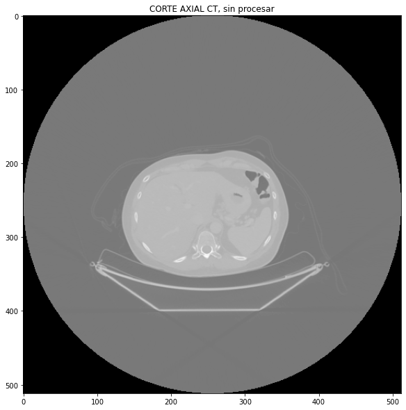
print(DCM.pixel_array)
[[-2000 -2000 -2000 ... -2000 -2000 -2000]
 [-2000 -2000 -2000 ... -2000 -2000 -2000]
 [-2000 -2000 -2000 ... -2000 -2000 -2000]
 ...
 [-2000 -2000 -2000 ... -2000 -2000 -2000]
 [-2000 -2000 -2000 ... -2000 -2000 -2000]
 [-2000 -2000 -2000 ... -2000 -2000 -2000]]
Ajustando la imagen#
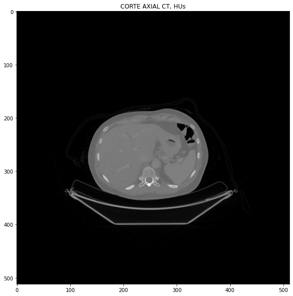
Obteniendo HUs#
Cada pixel de una imagen de CT corresponde a un determinado valor de unidades de Hounsfield. Sin embargo, los valores que se guardan en los archivos no corresponden directamente a los valores de HU, sino a una versión rescaleada (esto se debe básicamente a las limitaciones que impone el formato DICOM al tipo de dato a usar). Por eso, para obtener HU, es necesario aplicar la siguiente transformación lineal:
print(DCM.RescaleType)
print(DCM.RescaleSlope)
print(DCM.RescaleIntercept)
HU
1
-1024
imagen = DCM.pixel_array * DCM.RescaleSlope + DCM.RescaleIntercept
print(imagen)
[[-3024. -3024. -3024. ... -3024. -3024. -3024.]
 [-3024. -3024. -3024. ... -3024. -3024. -3024.]
 [-3024. -3024. -3024. ... -3024. -3024. -3024.]
 ...
 [-3024. -3024. -3024. ... -3024. -3024. -3024.]
 [-3024. -3024. -3024. ... -3024. -3024. -3024.]
 [-3024. -3024. -3024. ... -3024. -3024. -3024.]]
print(imagen[50,256])
print(np.min(imagen))
print(np.max(imagen))
imagen2 = np.clip(imagen, -1000,np.max(imagen))
print(imagen2)
-1000.0
-3024.0
1251.0
[[-1000. -1000. -1000. ... -1000. -1000. -1000.]
 [-1000. -1000. -1000. ... -1000. -1000. -1000.]
 [-1000. -1000. -1000. ... -1000. -1000. -1000.]
 ...
 [-1000. -1000. -1000. ... -1000. -1000. -1000.]
 [-1000. -1000. -1000. ... -1000. -1000. -1000.]
 [-1000. -1000. -1000. ... -1000. -1000. -1000.]]
fig_1 = plt.figure(1, figsize=[10,10])
img1 = fig_1.add_subplot(111)
img1.imshow(imagen2, cmap='gray')
img1.set_title('CORTE AXIAL CT, HUs')
plt.show()
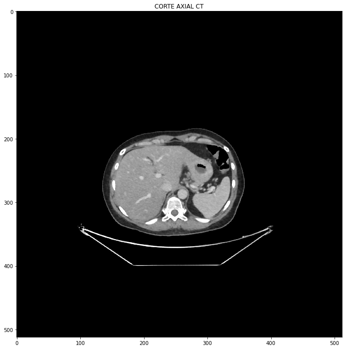
Window and Level#
El proceso de Windowing ( o grey-level mapping, contrast stretching, histogram modification, contrast enhancement, LUT, etc.) consiste en manipular las componentes de la imagen de forma tal que se puedan realzar ciertas estructuras particulares. El brillo de la imagen se ajusta a partir del Window Level, mientras que el contraste se ajusta a partir del Window Width.

Cada DICOM puede proveer un ancho y centro de ventana que viene desde el equipo de adquisición de imágenes:
print(DCM.WindowCenter)
print(DCM.WindowWidth)
40
400
Recordemos que el valor de los pixeles en el monitor van de 0 a 255
Típicamente si definimos
\begin{align} c &= \texttt{DCM.WindowCenter} \ w &= \texttt{DCM.WindowWidth} \end{align}
Entonces, la imagen transformada se obtiene como:
\begin{align} f_t(x,y) &= 0 &\textrm{si} \qquad f(x,y) < c - w /2 \ f_t(x,y) &= 255 &\textrm{si} \qquad f(x,y) > c + w /2 \ f_t(x,y) &= (f(x,y) - c) \times 255/w &\textrm{en otro caso} \end{align}
print('El centro de ventana es: ', DCM.WindowCenter, '\nEl ancho de ventana es: ', DCM.WindowWidth)
El centro de ventana es:  40
El ancho de ventana es:  400
Veamos si podemos hacer esto sin tener que generar otra imagen transformada. Para eso, veamos los parámetros opcionales de plt.imshow:
plt.imshow?
Es decir que si pasamos el máximo y el mínimo de la ventana, ya obtendríamos el resultado esperado:
c = 40
w = 400
ventmax = c + w/2
ventmin = c - w/2

fig_1 = plt.figure(1, figsize=[12,12])
img1 = fig_1.add_subplot(111)
img1.imshow(imagen, cmap='gray', vmin=ventmin, vmax=ventmax)
img1.set_title('CORTE AXIAL CT')
plt.show()
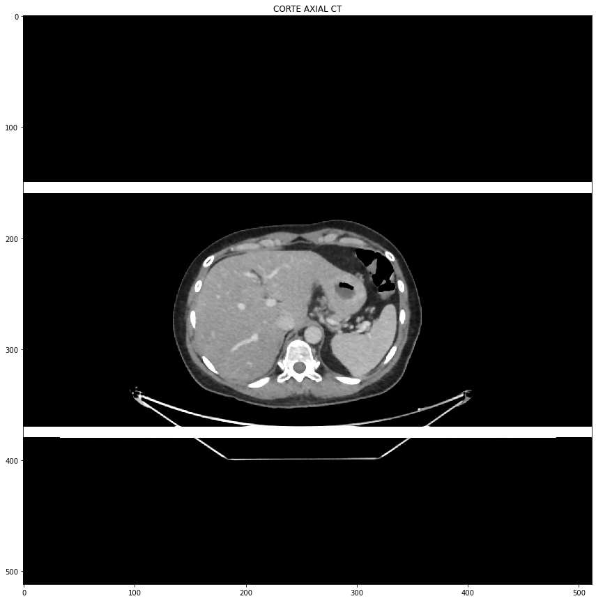
Manipulando la imagen#
Finalmente, podemos manipular la imagen a voluntad, dado que es un array de numpy. Por ejemplo, podemos reemplazar los puntos de la matriz por otros valores
imagen2 = imagen.copy()
imagen2[150:160,:] = 1000
imagen2[370:380,:] = 1000


fig_1 = plt.figure(1, figsize=[15,15])
img1 = fig_1.add_subplot(111)
img1.imshow(imagen2, cmap='gray', vmin=ventmin, vmax=ventmax)
img1.set_title('CORTE AXIAL CT')
plt.show()
O reemplazar ciertos puntos de acuerdo a una condición particular:
imagen2 = imagen.copy()
imagen2[imagen2 < -800] = 1000
fig_1 = plt.figure(1, figsize=[15,15])
img1 = fig_1.add_subplot(111)
img1.imshow(imagen2, cmap='gray', vmin=ventmin, vmax=ventmax)
img1.set_title('CORTE AXIAL CT')
plt.show()
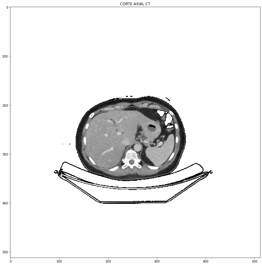
imagen2 = imagen.copy()
imagen2[(imagen2<-800) & (imagen2>-1100)] = 1000

fig5, g = plt.subplots(1, 2, figsize=[16,10])
g[0].imshow(imagen2, cmap = 'gray', vmin=ventmin, vmax=ventmax)
g[0].set_title('IMAGEN 2')

g[1].set_title('HISTOGRAMA de IMAGEN 2')
g[1].hist(imagen2.ravel(), bins=300) #ravel devuelve un vector 1D con todos los elementosde la matrix.
g[1].set_xlabel('HOUNSFIELD UNITS')
g[1].set_xlim()
g[1].set_ylim([0, 4000])

plt.show()

print('El FOV del CT del PET es de: ', imagen2.shape[0] * DCM.PixelSpacing[0], 'mm')
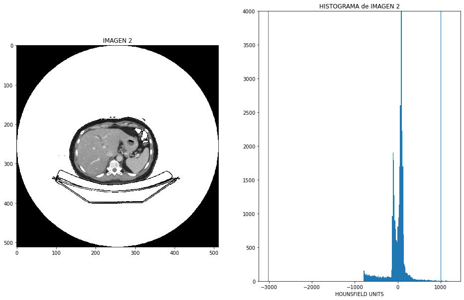
El FOV del CT del PET es de: 700.000256 mm
Ventanas de visualización típicas en CT#
Cabeza y cuello
cerebro w:80 c:40
subdural w:130-300 c:50-100
acv w:8 c:32 / w:40 c:40
hueso w:2800 c:600
Tejido blando: w:350–400 c:20–60
Pecho
Pulmones w:1500 c:-600
Mediastino w:350 c:50
Abdomen
Tejido blando w:400 c:50
Hígado w:150 c:30
Columna
Tejido blando w:250 c:50
Hueso w:1800 c:400